
SPSS Tutorials
The art of fetching useful insights from the data is now just not limited to the professional’s hand but modern tools like IBM SPSS are also capable of serving the best from a massive data set. Big organizations are using such tools to get valuable information from the data generated from multiple sources. Let’s see what is SPSS and how it is getting used in today’s work culture.
| In this SPSS Tutorial, we will go through below topics |
What is SPSS?
SPSS is a versatile program that was developed for managing statistical procedures. SPSS is the Statistical Package for Social Science and is used for the analysis of complex statistical data by researchers and organizations. This software package was launched in 1968 by SPSS Inc. But later in 2009, it was acquired by IBM. It was designed especially for the management and analysis of social science data.
Officially SPSS was given the name - IBM SPSS Statistics. But the people mostly call it SPSS. Whenever there is a task of social data analysis then first preference is always SPSS because of its user-friendly English-like command language. Its user manual is very simple to understand as it is straightforward and easy to get.
The application areas of SPSS are health research centers, marketing companies, government projects, education, data mining, etc. It is also used in survey organizations, data mining, and many other statistical analysis operations.
Most of the research companies use SPSS for the analysis of survey data so that they can get their desired output and can fetch useful insights from the data.
SPSS Data
SPSS Statistics data is stored in the data files which are specifically designed for being used by the IBM SPSS Statistics, In this section, we will discuss the different forms of data files and how to use these files.
Reading Data
You can simply import the data from various sources and also can enter it manually. Here, we will discuss how to read stored data from:
- Statistical data files of IBM and SPSS
- Database applications
- Spreadsheet applications
- Text files
Reading Statistical data files of IBM and SPSS
Data of IBM and SPSS statistical files are saved with the .sav extension. You can open the saved data by the following steps:
- Open the “Menu” and go to the “File” option.
- Select “Open”.
- Click on “Data”.
- Search for the file sample. sav and open it.
- The Data Editor displays the data in the file.
| Want to enhance your skills in dealing with the worlds best IBM, enroll in our SPSS Training |
Import Excel Database Into SPSS:
Consider the following steps to import Excel Database in SPSS:
- Open the “SPSS”.
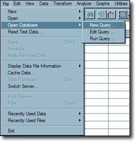
- Select the “File” menu.
- Click on the “Open Database” and select the “New Query” option.
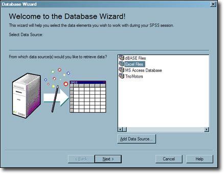
- SPSS Database Wizard will be open. Click on “Excel Files” in the selection window.
- Click on “Next”
- Select the “Browse” button in the ODBC Driver Login window.
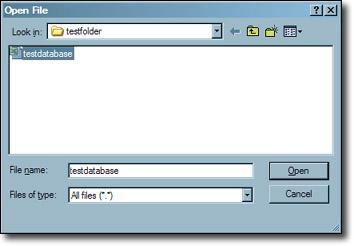
- Browse your required database file and then press enter on the “Open” button.
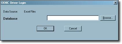
- Press “OK” to the ODBC Driver Login window.
- Select and drag the particular tables from the Available Tables box in the Select data window to the Retrieve Fields in This Order box.
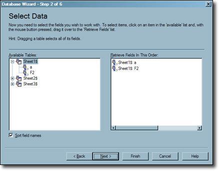
- Click on the “Next” button once all the tables are selected in the proper order.
- After this in the next step the Limit Retrieved Cases window will be opened.
- Here you can apply certain conditions to table variables. And, fields or functions can be added by drag and drop feature to expression within an expression cell.
- Press the “Next” button until you complete this window.
- Next, the Define Variables window will appear. In this, you can define the variables and assign them a name in the new SPSS file. Or else, SPSS uses the default names for the variables.
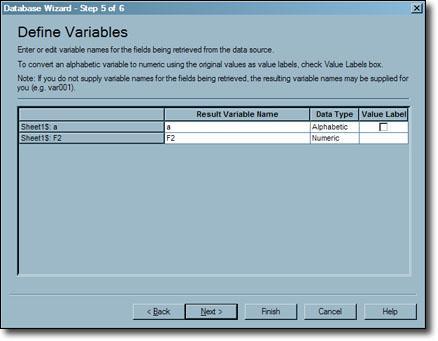
- Click on the “Next” button once you complete this window.
- “SQL Query window” will open after this. Here in the editor window, you can edit the SQL query string.
- Click the “Finish” button.
- Your Excel file will be imported and you can open it in SPSS.

Reading Data from a Database
From the database, the data can be imported using the Database Wizard which is not that complex. You simply need to install drivers for reading data directly from the database. The Open Database Connectivity (ODBC) driver is mostly used for this purpose and for different database formats. Any database with this driver can easily read the data. The installation CD is available for it. Other additional drivers are also available in the market by third-party vendors.
Example: Let us consider an example. It is based on Microsoft Windows and the driver in this is ODBC. This driver is only compatible with the 32-bit version of SPSS and IBM statistics. You can follow the same steps if you are using some other platform but you need a third-party ODBC driver to access it.
- Select the “File” menu.
- Open “Database” and select “New Query”
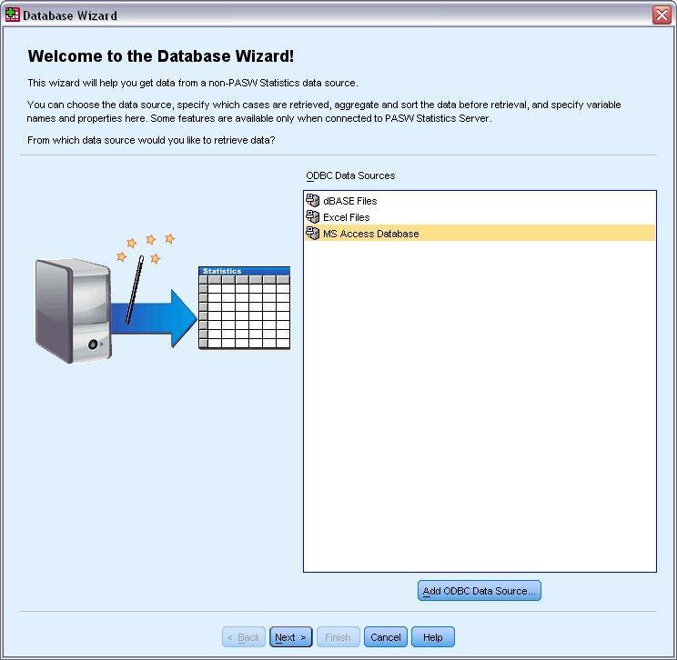
- Select “MS Access Database” from the list of data sources and click “Next”.
- Note to consider: On the basis of your installation, on the left side of the wizard, there may be a list of OLEDB data sources, in this example, we are using the list of ODBC data sources which is displayed on the right side of the wizard.
- Click on the “Browse” button to navigate to the Access database file and open it.
- Open the file named ‘sample.mdb’.
- Click “OK” in the login dialog box that appeared on the screen.
- After this, mention the tables and variables which you are supposed to import.
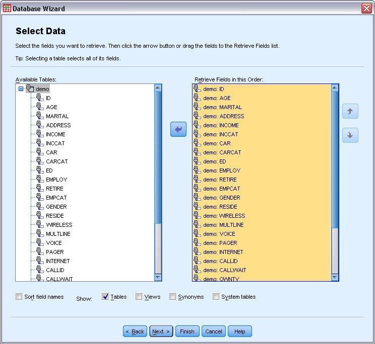
- Next step is to Drag the demo table to the Retrieve Fields.
- Click the “Next” button to move for the next step.
- In this step, select the required records to import from the database.
- You can use some of the cases from the database or you can say the subset of cases. Also, it is not necessary to import data serial-wise. You can import random data from the source.
- For the big database, you can limit the total number of cases to a small sample to minimize the processing time.
- Click the “Next” button to continue the process.
- Field names are preserved to create the variable names and also the variable names can be changed before import. If required then the names can be converted to valid variable names.
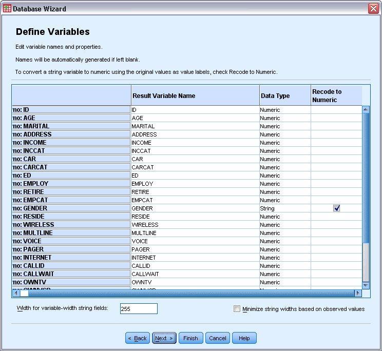
Define the Variables step
- In the Gender field, click on the Recode to Numeric cell. The variable can be converted from string to integer type. And, for the new variable, the original value will be retained as the value label.
- Press the “Next” button to continue.
- In the Result step, the SQL queries will be shown which were created in Database Wizard. Now you can run the statement or can save it to the file.
- Click the “Finish” button to import the data from the file.
- All of the data imported in the Access database is ready to use in Data Editor.
Reading Data from a Text File
In this section, we will discuss the steps to read a text file in SPSS. The text file is stored with the extension .txt. The file which we will consider in the example is named as awards.txt. It includes the following steps:
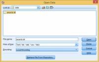
Select File Menu => Read Text Data
Browse the file that you want to read. The dialog box of the Open Data window appears.
Click the required file awards.txt and press the open button.
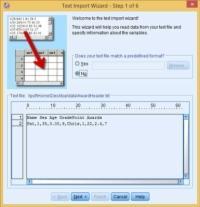
The Text Import Wizard will appear on the screen to load the data. Here, you can format the data to make it as per the requirement.
Check the input data and then press the Next button.
Verify the selected file to analyze whether the file is correct or not by checking the contents of the input file. If your file is already in a defined format then you can skip some of the steps and can select your file here. And, if it is not in a predefined manner then you can follow the further steps.
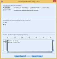
Mention that the data to read is delimited.
You can specify that the data in your file is organized and can be separated using tabs, space, and commas, etc. Maybe your data is already separated by having a fixed width and cannot be divided as data items are fixed together.
Click on the Next button.
Mention and check where the data are located in the file.
SPSS interpreting the text data.
You can specify to the SPSS the file which you want to read. And also, you will have one line of text representing the one row of data in the SPSS. Or you will have the SPSS count the variables to check from where the row is starting.
It is not required to read the whole file. You can randomly select the lines from a file or can select a percentage of the total lines in the file. This selection of lines will work as a test section and it is a very useful process if you are dealing with a large data file.
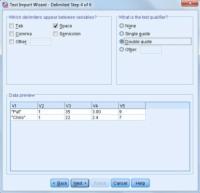
Click Next => define space as delimiters => double quotes as text qualifiers.
The SPSS knows very well that how to use the spaces, commas, tabs, etc., for the separation in the file. Some other characters can also be used as a delimiter by selecting the ‘Other’ option. Then you are able to write the character into the blank. You are enabled to define that your file text is formatted within the quotes. You can format your data by using both single and double-quotes. Strings should be written within quotes if they are containing any of the characters as delimiters.
The missing data item in the text file can also be specified in the file by using two delimiters.
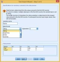
Press the Next button. Modify the variable name and if required change the format.
By default, SPSS will assign the names to variables like V1, V2, V3. You can change the variable name by updating the new name in the variable name field. From the data format drop-down list, you can also modify the data format.
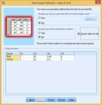
Click the Next button. Save format and also analyze the syntax
If you want to save the file for future purpose then click the no button to get the file save.
In SPSS this file will be used if you are going to upload a similar life with the same formatting. Next time when you load the file, it will save your time of formatting and reduce answering the questions again.
Press the Finish button.
The SPSS may take some time to finish the processing and this time depends on the formatting you have done on the data. And, your data will be displayed on the Data Editor Window.
Data View.
The file name will be asked and you need to enter the file name. You can call the name Awards. As the new file will be saved with extension .sav and it represents the SPSS file.
Reading the SPSS file is quite flexible as compared to the example shown. And, the reason will be explained with the second example. The file AwardHeader.txt contains the same data as the previous file but has different formatting.
In this file, the variable names will be mentioned in the first line. The whole data is placed in one line and is separated by commas. The data reading process is the same as we have done before. This time it will not be done in a single step as SPSS cannot predict the header and the data.
Modify data types and formats. Then Save File.
You are supposed to explain the data parts otherwise the data will remain like a block of text.
In the previous steps, it was explained that the SPSS is notified to show the variable name in the first line of the text file.
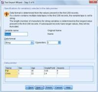
Step 3 of 6, the data starts from line 2 of the file. Every case is having five data items.
In the input text file, the data can be entered in the lower lines. But the variable names are entered in the first row of the file. SPSS may not read the starting and ending lines of the file but when it has a complete case it counts the data values.
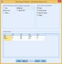
Specifying the delimiters. Put the characters in the quote.
In the previous steps, 4 of 6, commas and spaces were used as the delimiters in the file. As in this example, space was not used as a delimiter but there no problem if you want to use it. Here SPSS analyzes by itself that where space is required and applies the setting by default. And after that, it organizes the data as per the requirements defined by you. SPSS will read the variable names. Also, mention these names as the column headers.
Modify variable names and mention their types.
SPSS will automatically detect the type of variable name by itself.
After completion of Step 6 of 6, press the Finish and wait to get the data load.
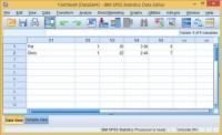
The data will appear in SPSS as you have formatted it.
| Check Out: SPSS Tutorials |
Using the Data Editor
Data Editor is used to displaying the data in the file. In the Data editor, the information is displayed in the form of the variables and the cases.
- In the Data View, variables are represented by the columns and on the other hand, cases are represented by the rows.
- And in the Variable View, each row is representing a variable, and each column is acting as an attribute which is associated with the respective variable.
Here the variables are used to show the different types of data which you have compiled. If we consider a survey then each question is equal to the variable. A variable can be a string, integer, date, currency, etc. It can be of any type.
The design of the Data Editor is similar to a spreadsheet. It has some differences which are mentioned below.
- Every single column represents the variable in your data.
- Each case is represented by the observation or case.
- Cells do not contain formulas. They include values only.
- In the dataset, the empty cell is considered as the missing value. That’s why there is no empty cell in the data table. But in the string cell, the blank is taken as valid.
Entering Numeric Data:
In the Data Editor, you are able to enter the data. This can be used for both small as well as the large file. For large files, it can be used to make small edits.
- At the end of Data Editor, there is the Variable View tab. Select it.
- Define the required variables which will be used. Here, in this example, three variables - ‘age’, ‘income’ and ‘marital status’ will be used
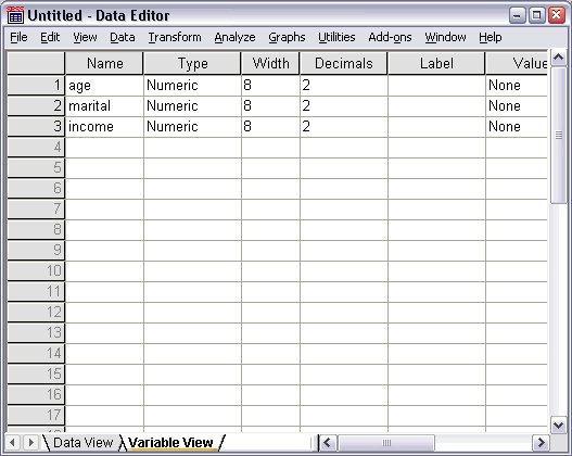
The Variable names in the Variable View
- Type age in the very first row of the first column.
- Then in the second row, type marital.
- And, in the third row, type income.
- A Numeric data type will be assigned automatically to the new variables.
- SPSS also generates unique variable names if not defined by the user. But these names not recommended and are not descriptive for the big data files.
- To continue the data entering, select the Data View tab.
- In the Variable View, the names that you have given are the headings for the first three columns in the Data View.
- Starting from the first column, you can begin to enter data in the first row.
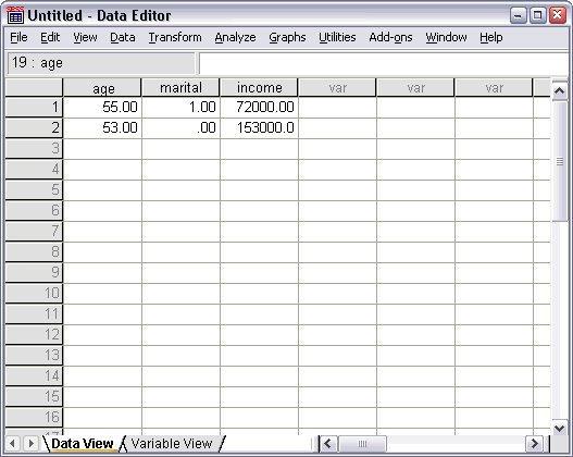
Values entered in the Data View
- Now, in the age column add value by typing 55.
- And in the marital column, type 1.
- Again, in the income column, type 72000.
- Go to the second row and add the data for the next subject.
- Again type 53 in the age column.
- And, in the marital column, type 0.
- In income column, type the value 153000.
- Here, the columns - age and marital show the decimal points, even when their values are supposed to be integers. And, to hide these decimal points in values of these variables:
- At the bottom of the Editor window, click on the Variable View tab.
- Then to hide the decimal, in the Decimals column of the age row, type 0.
- And also, in the Decimals column of the marital row, type 0.
Entering String Data
- In Data Editor you can enter the Non-numeric data like strings of text.
- There is a Variable View tab in the window. Click and select.
- Enter the variable name ‘sex’ in the first cell of the first empty row.
- Select the Type cell next to your data entry.
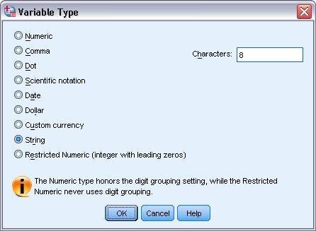
- On the right side of the Type cell, click at the button to open the dialog box of Variable Type.
- Select the String option to define the type of variable.
- Click the OK button to save your selection. And get back to the Data Editor to continue further.
Defining Data
In addition, to define the data types, you are free to specify the descriptive variable labels and also the value labels for variable names and data values. These defined labels can be used in statistical reports and charts.
Core Functions of SPSS
Four programs are offered by the SPSS that guides the researchers to deal with their complex data analysis requirements.
SPSS Statistics Program
The SPSS Statistics program facilitates a plethora of basic statistical functions. These functions consist of frequencies, bivariate statistics, and cross-tabulation.
SPSS Modeler Program
Modeler program for SPSS guides the researchers in performing their research operations like designing and implementing the predictive models with the support of advanced mathematical statistical measures.
Text Analytics for Surveys Program
For Survey program, SPSS Text Analytics helps the survey administrators. They represent the suggestions on the basis of the responses to the survey questions.
Visualization Designer
Visualization Designer program of SPSS enables the researchers to create a large variety of visuals easily such as radial boxplots by using their data.
The SPSS also includes solutions for data management processes which makes the complex programs simple. It makes the researchers able to perform the case selection, file reshaping and also to create derived data.
SPSS is the best solution for multiple tasks including data documentation. The researchers can easily save their confidential data as the metadata dictionary. And, this dictionary act as a centralized repository of information which is used at the runtime. It is pertaining to data like meaning, origin, format, and relationships with the other data.
Key Benefits of Using SPSS for Survey Data Analysis
For manipulation of the data, the usage of SPSS tool is one of the benefits that the researcher can take. It is best for the statistical analysis of survey data.
You can export any data in SPSS for the analysis purpose. The survey data gathered by SurveyGizmo can also be used.
This saved data file has .SAV extension and with this, you can apply the process of manipulation, data analysis, etc.
With this, the SPSS will automatically define the default variable names, types and the value labels. And also, it reduces the time and workload of the researchers. There is a number of features and opportunities for the users in SPSS.
SPSS is customizable and flexible so that you can use it as per your requirement. You can find the solutions for the complex datasets and can easily develop the predictive model.
For Individual Variable Examine Summary Statistics
In this section, the simple summary measures are discussed. And also, it includes how the level of measurement of a variable is influencing the types of statistics. Here, the data file names as demo.sav will be used.
Level of Measurement
There are different summary measures for different types of data and it depends on the level of measurement:
- Categorical – Categorical data means the data with a limited number of different values or categories. Also, it can be referred to as the qualitative data for the procedure works. These categorical variables can be the numeric variable or string data. The numeric variables use the numeric codes to show the different categories. Basically, there are two types of categorical data and these are mentioned below:
- Nominal – In this type of categorical data there is no inherent order for the categories. For instance, the job category of sales is not low or high than the job category of research.
- Ordinal – Whereas the Ordinal categorical data is that which has a meaningful order of categories. But there is no way to measure the distance between the categories. For instance, there is an order for the values as high, medium, and low. But again the "distance" is not measurable between the values.
- Scale – It means that the data is measured on a ratio scale. Here the data values represent both the distance and the order of values. For example, the salary of $72,195 is quite higher than the salary of $52,398. And also, the distance between the two variable values is $19,797. Also, it r also referred to as quantitative or continuous data.
Categorical Data Summary Measures
The most complex and difficult summary measure for categorical data is the number of cases for each category. The category mode is the one with the greatest number of cases. And, if the ordinal data has more categories then the median can be the beneficial summary measure for it. The median is the value where half of the cases fall above and below.
The frequency tables represent both the number and the percentage of cases for every single observed value of a variable. Frequencies procedure generates this table.
- Go to the menu and choose:
- Analyze => Descriptive Statistics => Frequencies
- Note: The Statistics Base option is required for this option.
- Select the Owns PDA and also the Owns TV. Move both of them into the list of Variables to process further.
- Press the OK button to run the procedure.
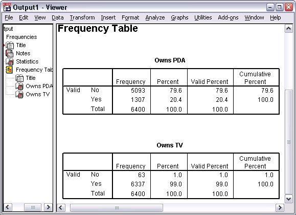
Frequency tables
The frequency tables can be viewed in the Viewer window. The frequency tables represent that only 20.4% of the person own PDAs. And, almost all the people (99%) owns a TV. This study may not be interesting but searching for those small groups of people will be interesting who do not use the TV.
Categorical Data Charts:
In a frequency table, the information can be displayed graphically with a bar chart or with a pie chart.
- Select and open the “Frequencies dialog box”. And, there you should select at least two variables.
- To get back to the recently used procedures you can use the “Dialog Recall” button.

- Click on the Charts.
- Select the Bar charts and then click on the Continue.
- Select the OK button to run the procedure in the main dialog box.
The frequency tables can also display the same information in the form of bar charts. It makes it easy for people to see because most of the people have TV rather than PDAs.
Summary Measures for Scale Variables
Several summary measures are available for scale variables. It includes:
- Central tendency measures - Mean and Median both are the most common measure for the central tendency
- Measures for dispersion - Statistics include standard deviation to measure the variation in the data.
- Again, open the “Frequencies dialog box”.
- To clear any previous settings, select the “Reset” option.
- Click and select the Household income in thousands [income] to move it in Variable list.
- Select “Statistics”.
- Click the “statistic measures” - Mean, Median, Standard deviation, Maximum and also the Minimum.
- Press the “Continue” option.
- Frequency tables are not much useful so deselect these tables
- To run the procedure, click the “OK” button.
The table of Frequencies Statistics will be shown in the Viewer window.
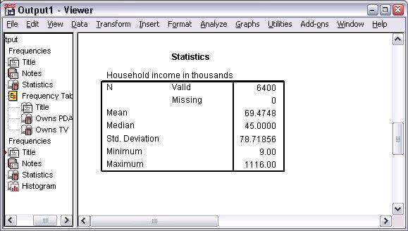
Table of Frequencies Statistics
Mean and Median both are the different measures. For example, the value of mean is about 25,000 times greater than the median value. It indicates that these values are not normally distributed. The distribution can also be check by the histogram.
Histograms for Scale Variable:
- First, open the “Frequencies dialog box”.
- Click the “Charts” option.
- Choose the Histograms with the normal curve for output representation.
- Click the “Continue” button. And, press button “OK”.
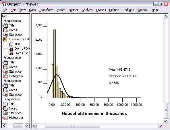
At the lower end of the scale, with the fall below 100,000, the majority of the cases are clustered. There are only a few cases in the range of 500,000 and beyond. These high values have more effect on the mean than the median. And it makes the median better statistic measure.
Time-Saving Features
This product comes loaded with a lot many features which can be really helpful when you are working on an analysis of data sets particularly when the analysis is being performed on a similar type of data sets.
Copying Data Properties
The data file in IBM SPSS contains the Metadata attributes which are linked with the data file that can be anything like variables, value labels or the missing value definitions, etc. So this avoids recreating the information every time you start working on a new data file. This can save a lot of time and you just need to copy the variable settings from a saved IBM SPSS Data file. The file properties from one file can be applied to the currently active dataset.
This method is helpful in:
- Creating new variables in the currently active dataset on the basis of external source data set file.
- Properties of some external variables can be applied to the active dataset variables.
- Properties of one external data set variable can be applied to multiple variables of the active dataset.
Displaying Data Dictionary Information
This contains the dictionary of information for the different variables for the active data file.
Information could be like:
- Variable Names
- Variable labels
- Measurement level
- Value labels
- Missing values
These are the steps you can refer to go to display Data Dictionary.
File > Display Data File Information > Working File...
This will display each variable with its specific properties. You can easily save this information in some output file or you can have that Information printed as a hard copy for your reference.
Dialog Recall
This button will show you the list of recently accessed dialog boxes. You can click this button to return to any listed dialog box.
This button looks like this:
This is helpful if you need to rerun some analysis or make some modifications to the existing analysis in the session and run.
Customizing IBM SPSS Statistics
This feature helps you to customize the user interface and this can really save a lot of time because it provides you easy access to the most frequently used features.
Creating Custom Menu Items
These Menu items can be easily created to run command syntax files, scripts. You can create your own menu with your choice of items.
Steps to go to Menu Editor: View > Menu Editor…
Here you can create your entire menu as per your choice or you can easily edit the existing one too.
Creating Custom Toolbars:
Custom toolbars provide you a quick way to perform specific tasks. Let’s say that you want to create a graph or a chart all this can be achieved with just a simple click of a toolbar button.
Steps for Creating Custom toolbar: View > toolbars > Customize…
This will show you all the toolbars which are available and can be used in the currently active window.
Creating Custom Dialogs
This can be used for generating command syntax. You can create your own version of a dialog for built-in IBM SPSS Statistics procedure. You can also create a user interface for any set of command syntax and that can be parameterized based upon user input.
Below are the steps for building your custom dialog:
- Within the IBM SPSS Statistics Menu, you need to specify the property of the dialog.
- You need to specify the controls that are building the dialog.
- You need to create a syntax template that specifies the command syntax which the dialog generates.
Once you are done with the above steps you can then begin using it. This can also be stored at some external source location and can be shared later with other users also.
Automated Production
Using Production Jobs IBM SPSS Statistics can be made to run in an automated fashion. This program runs unattended and will terminate after it executes the last command, so this helps you to perform other tasks while it is running. Production jobs can be scheduled to run automatically at scheduled times.
Let’s talk about analyzing weekly reports which we all know is a time-consuming process, So Production Jobs helps us out here.
Below are the ways in which we can make Production Jobs to run:
Interactively
In this, the program runs unattended in a separate session which could be on your local computer or on a remote server. If the program is running on your local computer then that must remain ON and connected to the server until the job is complete.
In the background on a Server
In this case, the program is running on a separate session on a remote server. So, your local computer doesn’t need to be kept ON or connected to the remote server. You can also fetch the results after some time.
Do keep in Mind that running a production job on a remote server requires access to the server that is running IBM SPSS Statistics Server.
Scoring Data with Predictive Models
Scoring is the term used here and which is referred to as applying a predictive model to a set of data. IBM SPSS Statistics can be used to build procedures such as regression, neural network, tree, clustering. The specifications for a model can be saved in a file and that can be used to reconstruct the model and can be used to generate predictive scores in other datasets. The file can be XML File or a compressed file (.zip file).
Scoring Process consists of the below steps:
- Build the Model and save the Model File
- Apply that Model to a different dataset.
Building a Predictive Model
IBM SPSS provides you numerous procedures for building predictive models. The Predictive models pick up the useful data and these models are trained to work on that useful data. If that model gives you accurate predictions then that can be used to score real data.
Historical data which is pre-aggregated is made to run through predictive models in IBM SPSS Modeler. If the predictions are accurate than can be used to create a runtime predictive model. Retraining of models is done by changing the behavior patterns.
IBM SPSS Modeler 15 User’s Guide lists down the information about the IBM SPSS Modeler
Applying the Model
Select the Scoring Wizard in the Utilities and choose the data model file which could be an XML File or a ZIP File. Select the Case from the Data Section which was created any by this the Model can be applied for the prediction work.
SPSS Syntax Introduction
SPSS Syntax is the language which contains the instructions for the data. These instructions are used to predict, analyze and modify the data.
How to Paste SPSS Syntax
Click on Analyze > Descriptive Statistics > Frequencies > Paste.
This will open up the Syntax Editor which holds the Instructions which were given in the Frequencies dialog. Then by running the commands, you have created you can get the data in the form of charts.
How to run SPSS Syntax
You can select the commands and click the “Run” Button.
Writing Simpler Syntax
A little practice in writing SPSS syntax will help to get good and really fast results.
How to get SPSS Syntax
The following ways can be used:
- Click on File => New => Syntax
- Using the “Paste” Button.
- Drag and Drop Syntax file to execute in Data Editor Window.
- Click and select the “New Syntax toolbar” icon.
Why Use SPSS Syntax?
- Syntax helps us to work really fast.
- If you are aware of the syntax then the mistakes can be corrected easily.
Basic Statistics Made Simpler
Here in this section of the post, we will discuss some of the mathematical statistics technique:
Frequency Distribution: This lets us know the number of distinct values in a variable and the number of times they occurred.
Z-Scores What and Why? : These are linearly transformed data values which have a standard deviation of 1 and mean of 0. These are also referred to as Standardized scores or data values which are given a common standard.
Standard Deviation: Standard deviation is a main statistical measure which gives value as output. This value tells us to what extent the number lie apart.
Crosstabulation
Crosstabulation is the method to measure the relationship in the two categorical variables. For instance, Gender is considered as a column variable and the Age is taken as a row variable. In the age category, you can display the number of males and females by developing the two-dimensional crosstabulation.
- Click and open “table builder”.
- In the table builder, Analyze the menu and also custom the Tables.
- Select the “Reset” button and delete any of the previous selections.
- From the variable list, you can drag and drop the Age category to the Row area.
- And also, drag the Gender to the Columns area on the canvas pane.
- Press “OK” and start creating the table.
A simple crosstabulation: The main factor is the money that people are going to spend on the product. Here, we will consider an example to show the relation between the Personal Digital Assistant (PDA) and the income level.
- Click the “Menu” and select: Analyze => Descriptive Statistics => Crosstabs
Note: the Statistics Base option is needed.
- Choose the Income category in thousands as the row variable.
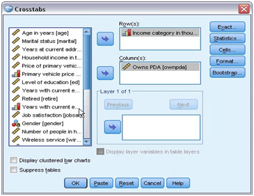
Crosstabs dialog box
- And also, choose the Owns PDA as the column variable.
- Run the procedure and press “OK”.
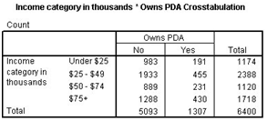
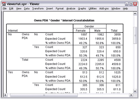
Crosstabulation table
In this table, the cells are representing the number of the cases for value joint combination.
Here the cells of the table are representing the number of cases for each joint combination of values. For example, 455 people fall under the category of the income in thousands i.e. $25,000–$49,000 own PDAs. And, the relationship between the variables is not indicated by the numbers in the table.
Counts vs percentage in crosstabulation: In each cell, it is quite difficult to estimate the crosstabulation. There are more than two crosstabulations as the several PDA owners come under the $25,000–$49,000 income category. Also, it is difficult for the ones who are under $25,000 income category as many people fall in this range.
- Open the “Crosstab dialog box” to proceed further.
- Use the “recall” button to return to the previous procedure.
- Click on the “Cells”.
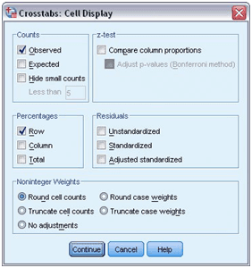
- In the Percentage group, clicks on the Row to check.
- Run the procedure by choosing continues option and then select “OK”.
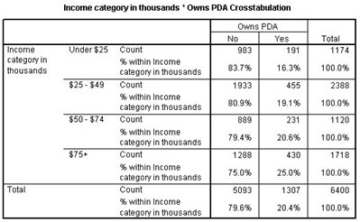
Crosstabulation with row percentages
In the above figure, it is clear that that the own PDA is increasing as the income increases.
Significance Testing for the Crosstabulation:
The key reason for evaluating the crosstabulation is to find the relation between the two variables. Many tests are there to find whether the relation between the cross-tabulated variables is significant or not. Chi-square is one of them and the benefit of using it is, it can be applied to various types of data.
- Again select and open the “Crosstabs dialog box”.
- Select “Statistics”.
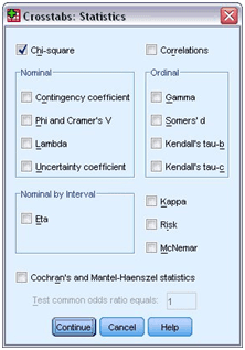
- Select and perform the “Chi-square test”.
- Select Continue and then “OK” to continue the process.
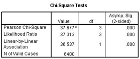
Pearson chi-square is used for hypothesis testing. It is done to estimate the relationship between the row and column variables and analyze that they are independent or not. We need the significance value as the actual value does not contain the information which we need. More the significant value is, more the variables are independent. Suppose if the significance value is coming as .000 then it means that the two variables are, indeed, related.
Add the Layer variable:
To develop a three-way table, you are allowed to insert a layer variable. In this, the row and column variables are further divided by the layer variable categories. It can also be called are the control variable because after adding a layer variable you can analyze the change in the relation of column and row variables.
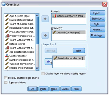
- Open “Crosstabs dialog box”.
- Select the “Cells” option.
- Remove Row Percents.
- Press “Continue”.
- As the layer variable select the Level of Education.
- Click “OK” and proceed further.
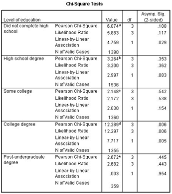
If you have a look at the crosstabulation table then you will notice that the table is large in size and difficult to analyze. And if you check the chi-square statistics table, it is easy to understand and interpret. In the education category, the apparent relationship between the two variables of PDA and income becomes negligible or disappears. This table mentions the relationship between the income column and the PDA owner.
| Related Article: SPSS Interview Questions |
Creating and editing charts
Multiple types of charts are available to create and use. You can use these charts to display your result of tasks. There are three most used charts which are mentioned below:
- Bar chart
- Pie chart
- Scatterplot with groups
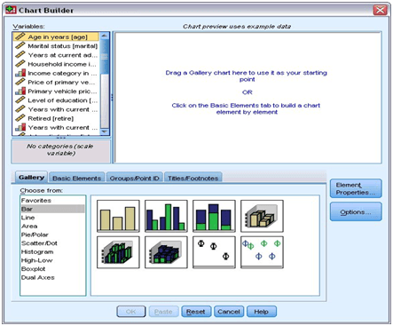
Chart creation basics
This section shows the basics of chart creation. Here, a bar chart is created which represents the mean income for different levels. In this example, a demo1.sav file is used.
Select the “Menu” option and choose: Graphs => Chart Builder
You can preview the chart while creating it and can modify it at the same time. You can view it in the Chart Builder dialog box which is an interactive window.
Working with Output
The result of your statistical procedure can be the tables, graphs, and charts, etc. It can be shown in the Viewer. It depends on you and your need that how you want to display the output means in the form of chart, text or table.
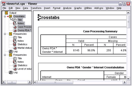
Using the Viewer
Viewer
The Viewer window is divided into two parts, one is the outline pane and the other is contents pane. Here the outline pane is used for an outline of the saved information and the contents pane includes the tables, statistical charts, and the text as a result.
You can explore the window’s content vertically or horizontally by using the scroll bar. Also, click on the item simply to display it in the contents pane.
- Change the width of the outline pane by clicking and dragging the right border. In the outline pane, there is an open book icon which shows that it is visible in the Viewer when it may not be visible in the contents pane.
- Double click on the book icon to hide the table. Then this open book icon will become the closed book icon. This closed book icon represents that the information is hidden and will not be displayed.
- Again, if you want to show the hidden information again then double click on the closed book icon. With this feature, you can also hide the complete data/ information.
- You can also hide the whole output from a particular mathematical-statistical process. The outline will get collapsed and it indicates that the output is hidden. You can modify the display order of the output.
- Click and move the items which are required.
- You can easily drag the items to a new location.
You can drag and drop the result items into the contents pane as per your requirement.
Using the Pivot Table Editor
Viewer
Creating a pivot table using pivot table editor is a simple task. With pivot tables, you can represent the results of your statistical procedures as shown in above figure.
TableLooks
The table is a way to represent your results in a proper format to make the result more clear and concise. Create the table in such a way that it will be easy to read and understand as it is a critical part of the process.
Using Results in Other Applications
You can use the results of this process in various applications like using table or chart in your report, documentation or presentations, etc.
Working with Syntax
You can run several tasks by simply using the command language. It helps you to store and automate the files. It offers a number of functions which are not available in the dialog box or the menu. These commands allow you to store your jobs for further use in the syntax file. You can use these syntax files to save your time when you will work on the same analysis of data.
The command language syntax file includes the IBM and SPSS statistics syntax commands and is a text file. You can directly type a command in a syntax window. You simply need to run the command and no need to perform many actions from dialog box or menu.
Pasting Syntax
Use the paste button to write the syntax. This button is available on the dialog box.
- Open the data file on which you want to perform operations.
- Select “Menu” and choose: Analysis => Descriptive Statistics => Frequencies
- Click the Marital status [marital]. Then drag it in the Variable list.
- Select the Charts.
- Click Bar chart option in the Charts dialog box.
- Select Percentages.
- Click the Continue button.
- Press the Paste option.
- Copy the syntax to the Syntax Editor.
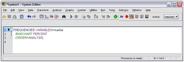
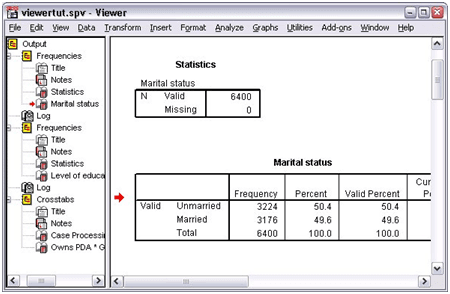
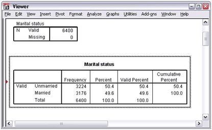
Frequencies syntax
- Run the syntax from the menu: Run => Selection
Editing Syntax
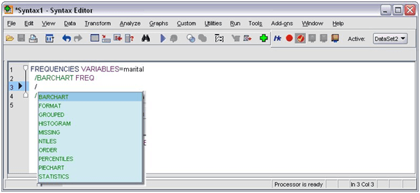
You can edit the syntax in the syntax window. You can modify the commands to represent frequency instead of the percentage. And also, you can directly enter the keyword for the frequency. Get the keyword by placing the cursor anywhere on the subcommand name. Then press the Ctrl+Spacebar and you will get the auto-completion control for the command. From the BARCHART subcommand, delete the PERCENT keyword. Then Press Ctrl+Spacebar together.
- For frequencies select the item labelled as FREQ. You can simply insert an item just by clicking on it. The item will be placed at your current cursor position.
The auto-completion control will provide you with the list of all available terms when you type.
- Click the “Enter” button after the “FREQ” keyword. Write the forward-slash which will show the start of the subcommand.
- In the Syntax Editor, you will get the subcommand list.
The F1 key is used to get the complete information about the current command. It will redirect you to the command syntax reference information. The syntax window shows the colored text which enables you to distinguish between the code easily. In this only the recognized coding terms are colored. If you make some spelling mistake while coding then you can easily identify it. Suppose if you have typed PRNT instead of PRINT command. PRINT command will be shown as colored by default whereas PRNT will be uncolored.
Open and the Run a Syntax File
- Open the saved syntax file by: File => Open => Syntax
A standard dialog box for opening files is displayed.
- Choose the file having .sps extension, you want to open and view.
- Select the “Open” button.
- Run the command using the “Run” option from the Menu.
If the command you are going to execute is applied to a specific data file. Then before you run the command, make sure that the data file is open. Or else you can open that file using the command.
Using Breakpoints
Breakpoints are used to stop the working of the code at the particular points and then you can run the code again when it will be ready. It makes you able to view the result at some point in the syntax and you can also get the current information by running a syntax command like FREQUENCIES. And, the breakpoints will be applied only at the particular level of commands. You cannot set it on any of the lines within the command.
How to Insert a Breakpoint in the Command:
- In the window, the breakpoint is represented by the red circle as you can see in the following picture. And you can click anywhere in the window region to the left of the text.
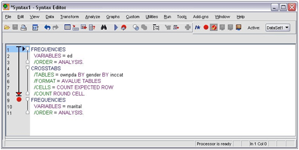
By the time you execute a syntax command which has breakpoints, the running process halts prior to every single command holding the breakpoint.
The progress of the executing command can be seen through the downward arrow pointing towards the left of the command text. It spans the first to last command of execution. It is very useful while executing command syntax having breakpoints.
To resume execution following a breakpoint:
- In Syntax Editor, click the “Menu”: Run => Continue
Modifying Data Values
In this section, we will understand why we need to modify the data. As we know, the information or data that we have to optimize may not be as per the requirement. So first we need to arrange it in a proper manner so that we can apply the procedure and model over it. Let us consider some examples:
- You want to create a categorical variable from the scale variable.
- To convert most of the result categories into a single category.
- If you want to create a new variable, this will be the calculated difference between the two existing variables.
- Measure the length of time between the two dates.
Creating a Categorical Variable from a Scale Variable
In the data file, most of the categorical variables are taken from the scale variables.
Several categorical variables in the data file demo1.sav is, in fact, derived from scale variables in that data file. These categorical variables include the integer values i.e. 1 to 4 which represents the income categories and this income is in thousands.
Steps to create the categorical variable - inccat:
- In Data Editor, open the “Menu” and choose: Transform => Visual Binning
In the Visual Binning dialog box, you can choose the ordinal variables and can create a new binned variable. Here, binning means combining two or more variables to make a group of the same category.
The visual binning depends on the value present in the data file and this will make you able to make the correct decision. For this purpose, you need to read out the complete file. It may be a time-consuming process as your file may have large cases. You can also scan the number of cases which are required to read. But it is not necessary in every case.
- You can simply drag the Household income in thousands. You can move it from the Variables list to the Bin list.
- Select “Continue”.
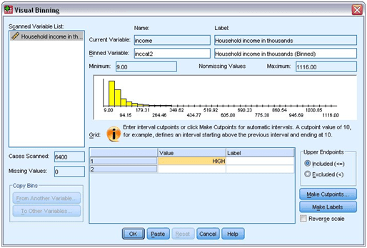
Main Visual Binning dialog box
- Click the Household income in thousands in the Scanned Variable List. You can clearly represent the distribution of the selected variable.
- To give the new binned variable name, you can enter inccat2. And for the variable label, enter the Income category [in thousands].
- Select and click “Make Cutpoints”.
- Choose “Equal Width Intervals”.
- Then for the first cutpoint location, enter 25 and 3 to give the number of cutpoints.
- Also, 25 for the width.
The number of cutpoints is one less than the number of binned categories. In the example, the binned variable has four categories and out of the first three include the range of 25 thousand. Where the last one will include all the values having the highest cutpoint value of around 75 thousand.
- Select “Apply”.
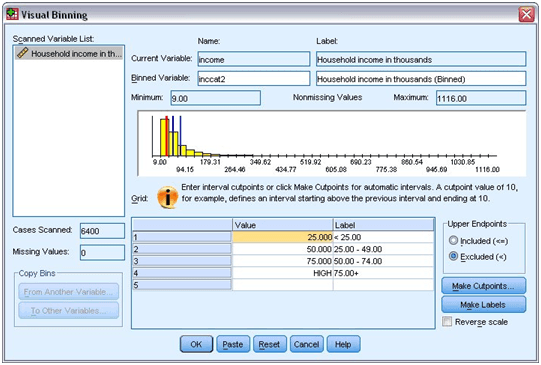
Now you will get values displayed in the grid and these values indicate the defined cutpoints. These cutpoints are the upper endpoints of categories. The locations of the cutpoints in the histogram indicated by the vertical lines.
- Choose “Excluded (<)” from the Upper Endpoints group.
- After that, click “Make Labels”.
Automatically generated value labels
It will automatically create descriptive value labels for each of the categories. The cutpoints and labels can also be added manually in the grid. You can also change its location by drag and drop line in the histogram.
- Select “OK”.
With this, a new variable will be created and it will be viewed in the Data Editor.
Computing New Variables
It is easy to solve and run complex equations by applying different statistical functions on the variables. Here in the example below, the difference between the two existing variables will be estimated.
In the file, there is a variable containing the respondent's current age and also the variable for years spent at current work. There is no variable consisting of time and age when the person starts his/her job. A new variable will be calculated which shows the difference between these two variables.
- Open the “Menu” and follow the steps: Transform => Compute Variable
- Type jobstart for the Target Variable,
- From the variable list, select the Age in years [age] variable. And, copy this variable to the Numeric Expression text box.
- In the calculator, press the minus key.
- Then select the variable for Years with current employer [employ].
- And, copy it to the expression.
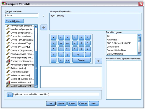
Compute Variable dialog box
- Select “OK”. With this, the new variable will be calculated here.
- The new variable is displayed in the Data Editor.
Working with Dates and Times
Date and time wizard is used to compute the tasks related to date and time data. You can easily perform these jobs using the wizard. With this wizard, you are able to execute the following tasks:
- You can create a variable for the date and time from a string variable.
- Also, the variables can be merged, having various information on date/time, to create a new variable.
- It makes you able to execute a task for adding or subtracting the values from date/time variables.
- And, you can also extract a specific part of a date/ time variable.
Use the Date or Time Wizard:
- Open the “Menu” and choose: Transform => Date and Time Wizard
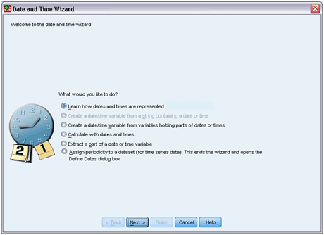
The screen shown in the above picture is showing general tasks set. The tasks which are not in use for the current data will be disabled. If you are working on it for the first time, then you get a brief overview by clicking the “Next” option. And also, from the help button, you will get complete information about the variables.
Conclusion
This digital era is revolving across the millions of data sources throwing information at an unstoppable pace. The requirement for tools like IBM SPSS is obvious for dealing with this information. Thus, you can get useful insights from your data and solve complex business problems by making quick decisions. This tools will help you to perform predictive analysis giving out effective and efficient results.
| Explore SPSS Sample Resumes Download & Edit, Get Noticed by Top Employers! |
 On-Job Support Service
Online Work Support for your on-job roles.

Our work-support plans provide precise options as per your project tasks. Whether you are a newbie or an experienced professional seeking assistance in completing project tasks, we are here with the following plans to meet your custom needs:
- Pay Per Hour
- Pay Per Week
- Monthly
| Name | Dates | |
|---|---|---|
| IBM SPSS Training | Jul 18 to Aug 02 | View Details |
| IBM SPSS Training | Jul 21 to Aug 05 | View Details |
| IBM SPSS Training | Jul 25 to Aug 09 | View Details |
| IBM SPSS Training | Jul 28 to Aug 12 | View Details |

Pooja Mishra is an enthusiastic content writer working at Mindmajix.com. She writes articles on the trending IT-related topics, including Big Data, Business Intelligence, Cloud computing, AI & Machine learning, and so on. Her way of writing is easy to understand and informative at the same time. You can reach her on LinkedIn & Twitter.


