
- SAP HANA Administration Tutorial
- SAP HANA Interview Questions
- SAP HANA Tutorial
- Application Programming Interfaces for SAP HANA
- Dell Introduces New Solutions for SAP HANA Environments
- Different Types of SAP HANA Modeling Views
- Fujitsu Services and Solutions SAP HANA Environments
- SAP HANA General Principles of Data Modeling
- SAP HANA Co-innovation for Real-Time Computing
- SAP HANA Data Modeling Tools Overview
- SAP HANA Database – SQL Script Guide
- SAP HANA Implementation and Useful Scenarios
- How to Build A SAP HANA Business Case for Your Investment
- How to Install SAP HANA Studio
- HP ConvergedSystem Solutions for SAP HANA
- Huawei SAP HANA Solutions Overview
- Introducing SAP HANA Extended Application Services (XS)
- Introduction to Application Development with SAP HANA
- Learn SAP HANA Use Cases for Your Industry
- Learn SAP HANA Studio Overview
- Making Big Data Real with SAP HANA
- NEC High-Performance Appliance for SAP HANA
- SAP’s Big Data Ecosystem Overview
- SAP Business Suite Powered by SAP HANA — Business Scenarios
- SAP Business Suite Powered by SAP HANA
- Learn SAP Business Warehouse Powered by SAP HANA
- SAP BW on HANA Implementation and Migration
- SAP BW on SAP HANA Administration
- SAP HANA Features and Building Blocks
- SAP HANA Integration with Microsoft Excel
- SAP HANA Introduction and Architectural Overview
- SAP HANA as a Primary ABAP Database
- SAP HANA Roadmap and Its Applications
- SAP S/4 HANA In Memory Basics and Projects
- Scoping Sizing Topics for SAP BW on HANA
- SAP HANA Specific Enhancements for SAP BW
- Steps to Create SAP HANA Application
- Steps to Create SAP HANA Business Case – Methodology
- System Landscape Options for SAP BW On HANA
- Using SAP HANA as a Secondary Database from ABAP
- VCE Vblock Specialized System for SAP HANA Architecture Overview
- What are the General Specifications of SAP HANA Hardware
- What are the HANA Skills Needed for Successful Projects
- SAP HANA Architecture Overview
- What is SAP HANA’s Big Data Strategy?
- What is SAP HANA Hardware?
- What is SAP HANA Rapid Deployment Solutions (SAP RDS)
- What is SAP HANA Starter
- SAP HANA Administration Interview Questions
SAP HANA Studio is an integrated development environment (IDE) used to develop and manage SAP HANA databases. It provides a graphical user interface (GUI) for creating, managing, and monitoring SAP HANA database objects such as tables, views, procedures, and functions.
HANA Studio is an integrated development environment (IDE) to develop artifacts in a HANA server. These artifacts may be Extended Application Services (XS), data modeling, or anything else that can be developed in HANA. However, to connect to the HANA server and develop, this IDE (HANA Studio) will need the HANA client installed. HANA Studio is a development program, much like Visual Studio, but the installed HANA Client enables the HANA Studio to connect to the server.
With SAP HANA Studio, developers can also create and debug SQL and Java scripts, perform data modeling, and administer security settings for SAP HANA databases. Additionally, SAP HANA Studio includes various performance optimization and troubleshooting tools, making it a comprehensive solution for SAP HANA database development and management.
About the SAP HANA Studio
SAP HANA Studio was first introduced in 2011 as the primary integrated development environment (IDE) for SAP HANA, a relational database management system developed by SAP SE.
At its introduction, SAP HANA Studio was considered a significant improvement over the previous tools used for SAP HANA development, which were based on Eclipse-based plug-ins. SAP HANA Studio was built on the Eclipse integrated development environment and provided a more user-friendly interface with advanced features that improved developers' efficiency and ease of use. Over time, SAP has continued to improve SAP HANA Studio by adding new features and functionality.
For example, in 2015, SAP introduced a new graphical modeling environment within SAP HANA Studio, allowing developers to create data models more efficiently. In 2016, SAP introduced a web-based development environment called SAP Web IDE for SAP HANA, intending to complement SAP HANA Studio. SAP Web IDE provides additional tools and functionality for developing and deploying SAP HANA applications in the cloud.
Despite introducing newer development tools, SAP HANA Studio remains essential for developers and administrators working with SAP HANA databases. It continues to receive updates and support from SAP and is widely used in many organizations that use SAP HANA. SAP HANA Studio is an essential tool for SAP HANA clients, developers, and administrators who work with SAP HANA databases. It provides a wide range of features that enable efficient and effective database development and management. Here are some of the key reasons why SAP HANA Studio is necessary -
- For providing a graphical user interface that makes it easy for developers to create, manage, and monitor SAP HANA database objects.
- For SAP HANA clients and developers to perform data modelling, which helps to create a logical representation of the database schema. This enables developers to understand the relationships between different data entities and optimize the database design for better performance.
- For allowing SAP HANA clients and administrators to manage user accounts and roles and define the security policies for SAP HANA databases.
- For optimizing performance through a wide range of tools for performance optimization, such as SQL and Java script editors, SQL query analysis, and performance trace analysis.
- For troubleshooting with a provision of a wide a range of debugging and troubleshooting tools that help developers to identify and resolve issues in their SAP HANA databases.
What is SAP Hana Studio?
SAP HANA Studio is an integrated development environment (IDE) used to develop and manage SAP HANA databases. It provides a user-friendly graphical user interface (GUI) for creating, managing, and monitoring SAP HANA tools and database objects such as tables, views, procedures, and functions. It also allows developers to develop and debug SQL and Java scripts, perform data modelling, and administer security settings for SAP HANA databases.
SAP HANA Studio is a comprehensive solution for SAP HANA database development and management, which includes a range of tools for performance optimization and troubleshooting. With SAP HANA tools, developers can efficiently create and manage their SAP HANA databases while ensuring high performance and security.
SAP HANA tool is an Eclipse plug-in known as an Eclipse-based tool. It serves two primary purposes, i.e., it is a central development environment known as an Integrated Development Environment (IDE). It is also an administration tool for both remote and local HANA systems. Also, it is a client tool that uses the client's end user to manipulate and manage data and applications deployed locally or in a remote setup.
| If you want to enrich your career and become a professional in SAP HANA, then enroll in "SAP HANA Training" - This course will help you to achieve excellence in this domain. |
Supported Platforms for SAP HANA Studio
The SAP HANA Studio is supported by various platforms. These are –
- Microsoft Windows x32 and x64 versions of – Windows XP, Windows Vista, Windows 7, Windows 8, and Windows 10.
- SUSE Linux Enterprise Server SLES 11 (x86 64-bit version).
- Red Hat Enterprise Linux (RHEL) 6.5
- Mac OS 10.9 or higher
- Eclipse platform 3.6
Features of SAP HANA Studio
- Sap Hana Studio Administration - This feature has tools for several administrative tasks. It also provides troubleshooting tools like the catalog browser, tracing, SQL Console, etc.
- SAP HANA Studio Database Development - It includes tools for database and content development. The devices are DataMarts, ABAP, etc.
- SAP HANA Studio Application Development - This includes SAP HANA native application development tools like XS and UI5 tools.

SAP HANA Studio Perspectives
SAP HANA Studio includes different perspectives that provide a customized user interface and tools tailored to specific tasks. Each perspective provides a specific set of features and tools that are tailored to the needs of developers and administrators working on SAP HANA databases. Users can switch between views based on the task at hand, ensuring an
efficient and effective development and management experience. Here is an overview of the different perspectives available in SAP HANA Studio -
- The SAP HANA Development perspective - This perspective is designed for developers and provides tools for creating, editing, and testing SQL and Java scripts, as well as for managing SAP HANA database objects such as tables, views, and procedures.
- The Debug perspective - This perspective is used for debugging and troubleshooting SAP HANA applications. It provides various debugging tools, including breakpoints, step-by-step execution, and variable inspection.
- The Modeler perspective - This perspective is focused on data modelling and provides tools for creating and managing SAP HANA data models. It allows developers to create a logical representation of the database schema, define relationships between data entities, and perform data validation.
- The Team Synchronizing perspective - This perspective is used for collaborative development and provides tools for managing source code, version control, and team synchronization. It allows developers to work together on SAP HANA projects while keeping track of changes and resolving conflicts.
- The Administration Console perspective - This perspective is designed for administrators and provides tools for managing SAP HANA databases and users. It allows administrators to manage security settings, configure system parameters, and monitor system performance.
SAP HANA Studio Environments
SAP HANA Studio provides several environments that allow users to perform specific tasks related to SAP HANA database development and management. Each environment provides a specific set of tools and features that are tailored to the needs of different users working on SAP HANA databases. Users can switch between settings based on the task at hand, ensuring an efficient and effective development and management experience. Here is an overview of the different environments available in SAP HANA Studio -
- Administration environment - This environment provides tools for managing SAP HANA system settings, configuring system parameters, monitoring system performance, and managing security settings. Administrators use it to manage SAP HANA databases and users.
- Information modeling environment - This environment provides tools for creating and managing SAP HANA tools like data models, including graphical data modeling tools, SQL editors, and tools for managing data types, views, and procedures. Developers use it to create and manage the database schema and data models.
- Data provisioning environment - This environment provides tools for importing data into SAP HANA databases from various sources, including SAP systems, non-SAP systems, and flat files. It includes tools for data extraction, transformation, and loading (ETL) and tools for monitoring data replication and synchronization.
- SAP HANA Database Administration environment - This environment provides tools for managing the SAP HANA database, including backup and recovery tools, performance tuning tools, and managing database storage and memory. Administrators use it to ensure SAP HANA databases' high availability and performance.
Download and Install SAP HANA Studio
Installation Path - The default installation on the system path according to OS and their version is -
- Microsoft Window (32 & 64 bit)- C:\Program files \sap\hdbstudio.
- Linux x86, 64-bit – /user/sap / HD studio.
- Mac OS, 64-bit – /Applications/sap / HD studio.app
Or, open the SAP Software Downloads, go to installations & upgrades if you still need to choose. Next, open > by Alphabetical Index (A-Z). After that choose H. Now, choose SAP HANA platform edition. Now, go to downloads if you still need to open it. And choose SAP HANA platform edition 2.0. Open downloads, if not already opened. Then, choose the installation. You can now download the items you need.
- Software Download - In the SAP Software Downloads, you can access the installation media and components for SAP HANA. In the SAP Software Hana studio Download Center, you find the media required to install a new SAP HANA system or to upgrade an existing one. Please note that all SAP HANA media on SAP Software Download Center are self-contained full installation media. This applies to the media available in the Installations & Upgrades and Support Packages & Patches sections. The section Installations & Upgrades only has media for the first revision of a Support Package Stack (SPS). The section Support Packages & Patches only includes the latest revision of an SPS. We strongly recommend using the most recent revision of an SPS to avoid running into already known and fixed issues. Therefore, by default, download media for all components of SAP HANA for an installation or upgrade from the section Support Packages & Patches.
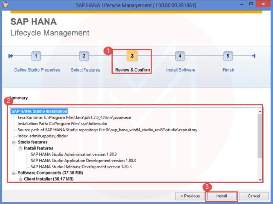
- Installation on Microsoft Windows – Initiate SAP HANA Studio installation in the default directory with administrative privileges or the user's home folder without administrative rights. Click on hdbsetup.exe to install SAP HANA studio.
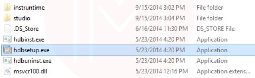
- Run SAP HANA Studio - Go to the Default installation folder "C:/Program Files / SAP / HD studio."There is an hdbstudio.exe file; you can create a shortcut on the desktop by right-clicking on it.
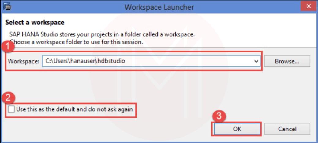
When you click the "hdbstudio.exe" file, it will open the Workspace Launcher screen as given in the picture, an SAP HANA Lifecycle Management Screen appears
- Workspace is selected by default. We can change the Workspace location by using the Browse option. Workspace is used to store studio configuration settings and development artifacts.
- Select the "Use this as the default and do not ask again" option to prevent the popup of this screen every time for workspace selection when we open SAP HANA Studio.
- Click the okay Button.
Key Features of SAP HANA Studio
SAP HANA Studio provides a comprehensive set of features tailored to the needs of developers and administrators working on SAP HANA databases. Here are some of the critical elements of SAP HANA Studio -
- Graphical user interface (GUI) - SAP HANA Studio provides a user-friendly GUI that allows developers and administrators to perform tasks such as creating and managing database objects, data modeling, and administering security settings.
- Data modeling - SAP HANA Studio provides various data modeling tools, including graphical data modeling tools and SQL editors, that allow developers to create and manage the database schema and data models.
- SQL and Java scripting - SAP HANA Studio includes tools for creating and debugging SQL and Java scripts, as well as for managing SAP HANA database objects such as tables, views, and procedures.
- Performance optimization - SAP HANA Studio provides tools for monitoring and optimizing the performance of SAP HANA databases, including tools for monitoring system performance, analyzing query performance, and identifying and resolving performance issues.
- Data provisioning - SAP HANA Studio includes tools for importing data into SAP HANA databases from various sources, including SAP systems, non-SAP systems, and flat files. It also contains tools for data extraction, transformation, and loading (ETL).
- Security Administration - SAP HANA Studio includes tools for managing user accounts and roles, defining security policies, and monitoring user activity to ensure the security of SAP HANA databases.
- Collaboration - SAP HANA Studio provides tools for collaborative development, including source code management, version control, and team synchronization.
Check Out: SAP HANA Interview Questions
Work With SAP HANA Studio
- Catalog - The Catalog represents SAP HANA's data dictionary, i. e. all data structures, tables, and data that can be used. All the physical tables and views can be found under the Catalog node.
- Provisioning - Data Provisioning, in simple terms, means bringing data or accessing the data from the source system to the target system without the interference of the data warehouse. So, the technique which we are using to fetch the desired data from the source to our target system is called Data Provisioning. There are four types of Data Provisioning Techniques in terms of the HANA point of view, which are as below -
- Real-time Provisioning
- Near Real Time provisioning
- Data Federation
- Local Data Import
So, let us see each provisioning technique in detail.
- Real-Time provisioning - This includes two tools. SLT (System Landscape Transformation and Replication Server) and Sybase Replication Server. These two tools are used for fetching real-time data/latest data from the source and paste in the target system with a latency of less than 5 seconds. Sources supported are SAP ECC and SAP Standard-supported Vendors (like Oracle. IBM, etc.)
- Near Real-Time Data Provisioning - Tools like BODS (Business Objects Data Services) and Informatica. BODS is an ETL tool that allows you to work on the metadata or data before pushing it to the HANA Target. It supports Structured and unstructured Data (Like HADOOP), and you can fine-tune the data as per your requirement before sending it to the target system.
- Data Federation - It is like Smart Data Access. In this case, we do not bring the data into the target system; we keep it where it is; we get the metadata and create the virtual data tables in the target systems. Then you can go on and build models on top of them, send them to the application layer, etc. This is achieved by installing drivers into the HANA box and being able to communicate with source systems like Oracle, Hadoop, MS-SQL Server, SAP HANA tools and system, Teradata, etc.
- Local Data Import - Since many business users use CSV and Flat files as a source, internally, SAP HANA tools has a local import that allows you to bring in CSV and Flat file data into the system.
- Content - The Content represents the design-time repository which holds all information on data models created with the Modeler. Physically, these models are stored in database tables visible under Catalog. The Models are organized in Packages. The Contents node provides a different view of the same physical data. The created Column Views are always located in schema _SYS_BIC, their metadata in schema _SYS_B.
- Security - SAP HANA Security protects essential data from unauthorized access and ensures that the standards and compliance meet as security standards adopted by the company. SAP HANA provides a facility, i.e., a Multitenant database, in which multiple databases can be created on a single SAP HANA System. It is known as a multitenant database container. So, SAP HANA provides all security-related features for all multitenant database containers. SAP HANA tools of security provide various security-related features such as user and role management, authorization, authentication, encryption of data in the Persistence Layer, and encryption of data in the Network Layer
SAP HANA Studio Frequently Asked Questions
1. What is SAP Hana Studio?
SAP HANA Studio is an integrated development environment (IDE) used to develop and manage SAP HANA databases. It provides a graphical user interface (GUI) for creating, managing, and monitoring SAP HANA database objects such as tables, views, procedures, and functions.
2. What is the use of HANA studio in SAP?
The HANA studio is a collection of applications for SAP. It enables technical users to manage the SAP HANA database, to create and manage user authorizations, and to create new or modify existing models of data in the SAP HANA database. It is a client tool, which can be used to access local or remote SAP HANA databases.
3. Which based tool is SAP HANA studio?
SAP HANA studio is an Eclipse-based tool. SAP HANA studio is both, the central development environment, and the main administration tool for HANA system. Additional features are − It is a client tool, which can be used to access local or remote HANA systems.
4. What are the perspectives and views of SAP HANA studio?
SAP HANA Studio includes different perspectives that provide a customized user interface and tools tailored to specific tasks. Each perspective provides a specific set of features and tools that are tailored to the needs of developers and administrators working on SAP HANA databases. Perspectives in the SAP HANA studio are the Development perspective, Debug perspective, and Modeler perspective.
5. What are the features of HANA studio?
A graphical user interface is a top feature. SAP HANA Studio provides a user-friendly GUI that allows developers and administrators to perform tasks such as creating and managing database objects, data modeling, and administering security settings. Data modeling is again a key feature. SAP HANA Studio provides various data modeling tools, including graphical data modeling tools and SQL editors, that allow developers to create and manage the database schema and data models. SAP HANA Studio includes tools for creating and debugging SQL and Java scripts, as well as for managing SAP HANA database objects such as tables, views, and procedures. SAP HANA Studio provides tools for monitoring and optimizing the performance of SAP HANA databases, including tools for monitoring system performance, analyzing query performance, and identifying and resolving performance issues. SAP HANA Studio includes tools for importing data into SAP HANA databases from various sources, including SAP systems, non-SAP systems, and flat files. It also contains tools for data extraction, transformation, and loading (ETL). Security Administration - SAP HANA Studio includes tools for managing user accounts and roles, defining security policies, and monitoring user activity to ensure the security of SAP HANA databases. SAP HANA Studio provides tools for collaborative development, including source code management, version control, and team synchronization
6. What are the requirements for SAP HANA studio?
The requirements for SAP HANA Studio may vary depending on the version of SAP HANA Studio being used and the size and complexity of the SAP HANA database being managed. It is recommended to check the official documentation of SAP HANA Studio for the specific system requirements for the installed version. Some minimum requirements include operating systems like Windows, Linux, or Mac OS X, minimum memory of 4 GB of RAM, and 8 GB or more recommended, minimum disk space of 2 GB of free disk space, Java runtime environment - Java 8 or higher version must be installed a 1024x768 or higher resolution display, and SAP HANA database version 1.0 SP6 or higher, or SAP HANA Express Edition.
7. How do I add a system to HANA studio?
To add a system to SAP HANA Studio, first open SAP HANA Studio and click the "Systems" tab in the "System Navigator" pane on the left-hand side. Next, right-click on the "Systems" folder and select "Add System" from the context menu. After that, in the "Add System" dialogue box, enter the system details, such as the system's name, hostname or IP address, and instance number. Next, select the appropriate security option, such as "Basic" or "SAPLogon Ticket", depending on the security settings of the system being added. Then click the "Advanced" button to set additional properties like SSL settings, time-out values, etc. Next, click the "Test Connection" button to verify the connection to the system. Lastly, click the "Finish" button to add the system to SAP HANA Studio. Once the system is added, it will be displayed in the "Systems" folder in the System Navigator pane. You can now use SAP HANA Studio to manage the system and perform tasks such as creating or modifying objects, monitoring performance, and deploying applications.
8. How to connect to HANA database from HANA studio?
To connect to a HANA database from SAP HANA Studio, first open SAP HANA Studio and go to the "Systems" view in the System Navigator pane. Next, expand the system you want to connect to and right-click on the "SAP HANA" node. Then select "Open SQL Console" from the context menu. After this, in the SQL Console dialogue box, enter your credentials for the HANA database in the "Authentication" section. Then select the database you want to connect to from the "Database" dropdown list. Lastly, click the "Connect" button to connect to the database. Once the connection is established, you can run SQL queries, create database objects, and perform other database administration tasks using SAP HANA Studio. You can also use the "Modeler" perspective in SAP HANA Studio to create and manage database schemas, tables, views, and other objects.
9. How do I find tables in HANA studio?
To find tables in SAP HANA Studio, first open SAP HANA Studio and connect to the system you want to search for tables. Go to the "Catalog" view in the System Navigator pane on the left. Next, expand the design and the schema under which you want to search for tables. Then right-click on the "Tables" folder and select "Open Object Search" from the context menu. Now, in the "Object Search" dialogue box, select the "Table" option from the "Type" dropdown list. Enter the name or a part of the name of the table that you want to search for in the "Name" field. Lastly, click on the "Search" button to start the search. The search results will display the tables that match the search criteria. You can then select a table from the search results and view its details, such as column names, data types, and indexes, in the "Columns" and "Indexes" folders in the "Catalog" view.
10. What is the difference between HANA client and studio?
The main difference between SAP HANA Client and SAP HANA Studio is their purpose and functionality. SAP HANA Client is a software package that provides the necessary libraries and utilities to connect to and interact with an SAP HANA database. It is a command-line tool that allows access to various database administration and application development tasks, including executing SQL queries, creating database objects, and managing database connections. On the other hand, SAP HANA Studio is a graphical user interface (GUI) tool that provides a comprehensive set of development, administration, and monitoring features for SAP HANA databases.
Conclusion
Overall, SAP HANA Studio provides comprehensive features that allow developers and administrators to efficiently create, manage, and optimize SAP HANA databases while ensuring high performance, security, and collaboration. With its user-friendly interface, data modeling tools, performance optimization features, data provisioning tools, and security administration tools, SAP HANA Studio has become an essential tool for organizations that use SAP HANA. Despite introducing newer development tools, SAP HANA Studio plays a vital role in the SAP HANA ecosystem. It is expected to remain an essential tool even in the near future. If you want to enrich your career and become a professional in SAP HANA, then enroll in "SAP HANA Training" - This course will help you to achieve excellence in this domain.
 On-Job Support Service
Online Work Support for your on-job roles.

Our work-support plans provide precise options as per your project tasks. Whether you are a newbie or an experienced professional seeking assistance in completing project tasks, we are here with the following plans to meet your custom needs:
- Pay Per Hour
- Pay Per Week
- Monthly
| Name | Dates | |
|---|---|---|
| SAP HANA Training | Jul 21 to Aug 05 | View Details |
| SAP HANA Training | Jul 25 to Aug 09 | View Details |
| SAP HANA Training | Jul 28 to Aug 12 | View Details |
| SAP HANA Training | Aug 01 to Aug 16 | View Details |

I am a passionate content writer at MindMajix. I write articles on multiple platforms such as Power BI, Blockchain, Fintech, Machine Learning, Artificial Intelligence and other courses. My work covers a variety of niches including the IT industry, E-commerce, education, fashion, product descriptions, well-researched articles, blog posts, and many more. Basically, I put love into words and help you connect with the people + moments that matter. You can find me on my Linkedin.


